Step-by-Step Guide for Beginners
At this point, we’ve all heard a lot about Quant investing and probably even invested in some Quant-based fund. So as the market makes new bottoms every day and as my portfolio bleeds further, I decided that this might be a good time to get my hands on something new.
I had some prior experience working on Python, mainly integrating it with finance in some form, and so exploring quantitative finance was on my to-do list since a long time. I think this is a good time to start.
In this blog, I’m going to write about something that I find pretty interesting: Backtesting a strategy. Mind you, this is a rather new domain for me compared to stuff I’ve covered in previous blogs, so it might not be perfect—but I’ll try my best.
Click here
Alright! So assuming you now have Python ready to go, let’s get started!
What is Backtesting?
Backtesting is the process of evaluating a trading strategy using historical data to determine its effectiveness before applying it in live markets. It allows traders and investors to simulate trades based on past price movements to assess profitability and risk.
It basically tells you how good or bad a strategy would have performed in the past, and considering that the markets often repeat themselves, I’d say that if something worked superbly in the past, it has a fairly decent chance of working in the future as well.
Key Python Libraries for Backtesting
We’ll be using the following libraries, which you can install using:
pip install yfinance pandas matplotlib backtrader
- Pandas: Handles time-series data using DataFrames.
- NumPy: Helps with numerical operations and vectorized computation.
- Matplotlib: For plotting price data and signals.
- yFinance: To fetch stock data from Yahoo Finance API.
- Backtrader: Main framework to run the backtest with built-in indicators and simulation capabilities.
We’ll use the classic “Golden Crossover” strategy for this blog: go long when the 50-day moving average crosses the 200-day moving average from below.
Step 1: Fetching Data
import yfinance as yf
import pandas as pd
import matplotlib.pyplot as plt

ticker = 'RELIANCE.NS'
data = yf.download(ticker)
data.columns = data.columns.get_level_values(0)

if data.empty:
    raise ValueError(f"Failed to fetch data for {ticker}. Check ticker symbol or connection.")
Step 2: Computing Indicators
This is optional, as Backtrader has built-in indicators. But you can still try it manually:
data['SMA_50'] = data['Close'].rolling(window=50).mean()
data['SMA_200'] = data['Close'].rolling(window=200).mean()
Step 3: Buy/Sell Signals
data['Signal'] = 0

data.loc[data['SMA_50'] > data['SMA_200'], 'Signal'] = 1

data.loc[data['SMA_50'] < data['SMA_200'], 'Signal'] = -1
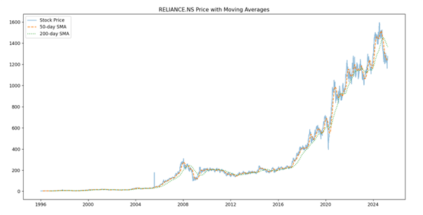
Step 4: Visualizing the Strategy
plt.figure(figsize=(12,6))
plt.plot(data['Close'], label='Stock Price', alpha=0.5)
plt.plot(data['SMA_50'], label='50-day SMA', linestyle='dashed')
plt.plot(data['SMA_200'], label='200-day SMA', linestyle='dotted')
plt.legend()
plt.title(f'{ticker} Price with Moving Averages')
plt.show()
Step 5: Using Backtrader
import backtrader as bt

class SMACrossover(bt.Strategy):
    def __init__(self):
        self.sma50 = bt.indicators.SimpleMovingAverage(self.data.close, period=50)
        self.sma200 = bt.indicators.SimpleMovingAverage(self.data.close, period=200)

    def next(self):
        if self.sma50[0] > self.sma200[0] and not self.position:
            self.buy()
        elif self.sma50[0] < self.sma200[0] and self.position:
            self.sell()
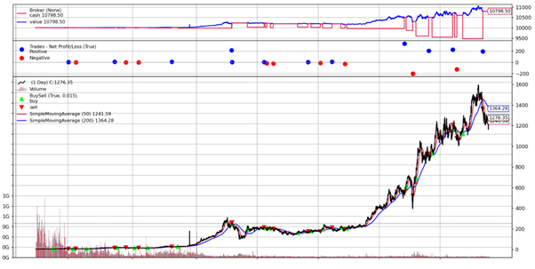
Step 6: Running the Backtest
cerebro = bt.Cerebro()
datafeed = bt.feeds.PandasData(dataname=data)
cerebro.adddata(datafeed)
cerebro.addstrategy(SMACrossover)
cerebro.run()
cerebro.plot()
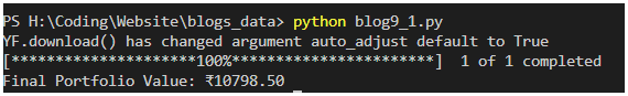
portfolio_value = cerebro.broker.getvalue()
print(f'Final Portfolio Value: ₹{portfolio_value:.2f}')
Conclusion
So that’s it—we successfully backtested our first strategy! If you followed along, you should’ve seen your own results as well.
This is just the beginning. In the next blog, we’ll go deeper by:
- Calculating returns and drawdowns
- Adding more indicators like RSI & MACD
- Optimizing strategy parameters
Stay tuned!